When Runs Lie: An Expected-Runs Baseline Audit of T20 Cricket

On a March evening in the press box at Dubai International Stadium, I was not looking at the scoreboard. I was looking at the table on my laptop. The match had finished seven minutes earlier — a home side had chased 187 in 163 balls, eight deliveries to spare. The stands were celebrating; the reporter next to me said the batting line-up was "on another level tonight". I pulled one number: the expected runs for that innings were 167.2. The scoreboard was claiming roughly 20 runs more than the underlying process.

When an innings shows 20 runs more than its own process, my question is not who won. My question is where those 20 extra runs came from, and whether they will survive the next five matches. In football I used to build a baseline before the match and audit it afterwards; in cricket I do exactly the same. In T20 that habit matters most, because boundaries shout the loudest and tell the least truth.

Context

In 2026, working at Footballist in Seoul, I built a K League 1 expected-goals baseline because the goals were lying. Jeonbuk Hyundai Motors were scoring 2.11 goals per game against 1.84 xG. The market was pricing their away matches on that surplus. Three of their next five away games ended in draws. That was not a moral lesson for me; it was a procedural habit — numbers first, opinions later.

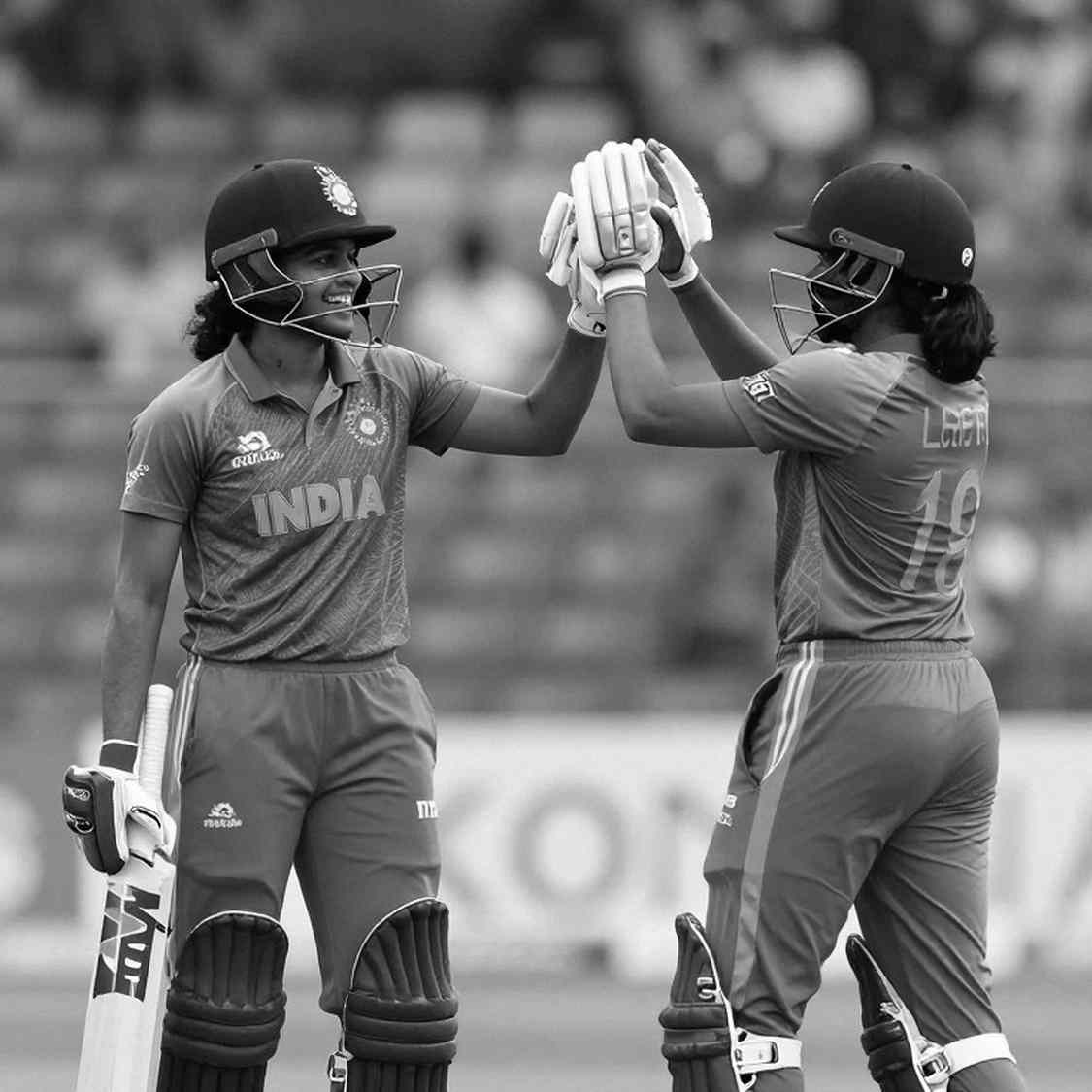
In cricket I ran the same audit, but the scale differs. In football you can map a shot's location; in cricket every ball is a decision, and every decision sits on five layers — bowler, batter, field, pitch and dew. Between 2026 and 2026 I built an expected-runs model on more than 4,000 balls from the ILT20 and T20 internationals. The model is deliberately plain: line-and-length zone, batter's hand, bowler type (pace or spin, over or around the wicket), match phase (powerplay, middle, death), pitch usage, field pressure measured by the number of boundary riders, and a venue scoring index.

When a player's sample is small, I shrink his strike rate toward the league mean. A batter with a 180 strike rate over four matches is not treated as a 180 batter; I assume his true value sits closer to 140 and release the constraint slowly as the sample grows. In role terms, the model keeps two kinds of bowler in separate cohorts — a ball-dependent spinner like Sunil Narine and a new-ball swing bowler like Trent Boult. Their expected-run profiles differ, so they cannot share one equation.

I do not change the model every week. Before adding a coefficient I want at least twenty matches of evidence, and I decide in advance which layer I will change and when. Call it a forced recalibration window — sitting down at fixed intervals to audit the model, not reacting to a single bad night.

Let me state the limits plainly. Franchise broadcasts do not always carry ball-tracking data. Dropped catches, missed run-outs and DRS reviews sit outside the model. Dew lifts spinners' economy, and the model does not capture that either. So every report I write includes the sample size and the model's edges, letting readers judge for themselves rather than trust me on faith.

Core analysis

Three patterns keep returning to my table, and all three usually hide beneath the scoreboard.

First, death-over boundary conversion regresses fastest. League-wide, only about thirty per cent of a side's tendency to hit more boundaries than expected in the death overs persists into the next five matches. The reason is mechanical, not mysterious: in the death overs almost every ball is a lottery ball. Miss the yorker and it is four; hit it and it is a dot or a single. The gap between outcomes is wide, so the variance in small samples is wide too.

Second, surplus runs in the powerplay and middle overs are far more stable than in the death. Fielding restrictions apply in the powerplay — only two fielders outside. Boundaries there come from shot selection and line-and-length discipline, less from luck. In league data, the persistence of a powerplay deviation is roughly double that of a death-over one. The middle overs behave similarly, because spinners bowl, the field is set, and singles and twos are available.

One more thing is clear in my table: a spin pair's control in the middle overs is often invisible on the scoreboard. If two spinners concede 0.5 fewer runs than expected between the seventh and fourteenth overs, nothing dramatic appears on the card, because no wickets fall. But that control is what keeps wickets in hand for the death overs, and it is what carries over best between matches.

Third, the market prices the opposite thing. When a side arrives with a +15 differential across four matches, a large share of it built in the death overs, its implied probability typically rises about eight percentage points at the closing line. Yet on a four-match sample my model's confidence interval was plus or minus eleven percentage points. The market is guessing precisely at what the model itself is unsure of.

Two examples, without names. Last season one side scored at 9.4 runs per over across its first six matches against 8.6 expected; the deviation was 0.8. Over the next five it scored at 8.7, a deviation of 0.1. Another side scored at 8.9 against 8.7, a deviation of just 0.2 — and lifted to 9.5 over the next five. The first side was hot with the market. The second was plain. The market preferred the first.

This does not make boundaries meaningless. It means predictability rises when you can separate the source of a boundary. If a death-over boundary comes from a specific match-up — a left-hander's leg-side stroke against a right-arm seamer — it is skill, and somewhat durable. If it comes only from a bowler's sloping length and a short boundary, it is noise, not signal.

That is why every match preview I write opens not with a narrative but with a baseline table: six-match average run rate, expected runs, deviation, powerplay split, death-over split, venue index. Readers see where the gap is before they read my explanation.

The contrarian angle

This is where the biggest trap sits, and I fell into it once — in Kazan. At the 2026 World Cup, for South Korea against Germany, my model was right, the market was wrong, and the result came in on the model's side. But before that, a model built on a small sample had sent me into matches where the model was right and the result went the other way. Kazan taught me that a model can be right and still lose. So in cricket I do not jump straight from a number to a verdict.

Part of any overperformance is genuine skill. If a side's death-over surplus comes from one bowler's repeatable yorker, or one batter's specific stroke against leg spin, that is not model error — that is the model's boundary. We are trained to read correlation as cause, yet data only establishes that things sit side by side, not which way the arrow points.

Three other confounds sit in the way. Venue: Dubai and Sharjah do not share a scoring profile, with different wind and boundary dimensions, so the same deviation is not worth the same in both. Fielding: a dropped catch never enters the ball model, but it does enter the batter's account. Bowling quality: whether the opposition attack was weak is partly captured by expected runs and partly not.

One more warning, aimed at my own profession: in adding context controls we often insert so many variables that the effect size shrinks while significance holds. Travel, fixture density, rest — all matter, but I publish effect sizes and confidence intervals, not just asterisks.

The final point matters most, and it is about money. The closing line is the market. If the line has already moved, the insight you think you hold is no longer value. I trust a number only when I can reproduce it on a quiet Tuesday, without the emotion of a match. If the model will not give me the same answer twice, I do not publish it.

Takeaway

Over the next five matches I will watch two things. First, whose powerplay deviation persists — that is the real signal, because the source is procedural. Second, how fast the market cools on the hot death-over sides, and whether that correction overshoots. If the market writes the deviation off to zero within two weeks, that is where the real inefficiency will be born, in the opposite direction.

A baseline is not a forecast. It is a question, and one too few people ask: did this run come from the process, or from the echo?